Here we examine the displacements and pressure variations associated with a sinusoidal sound wave traveling through air. Figure 17-5a displays such a wave traveling rightward through a long air-filled tube. Recall from Lesson 16 that we can produce such a wave by sinusoidally moving a piston at the left end of the tube (as in Fig. 16-2). The piston’s rightward motion moves the element of air next to the piston face and compresses that air; the piston’s leftward motion allows the element of air to move back to the left and the pressure to decrease. As each element of air pushes on the next element in turn, the right–left motion of the air and the change in its pressure travel along the tube as a sound wave.
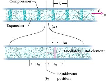
Fig. 17-5 (a) A sound wave, traveling through a long air-filled tube with speed ν, consists of a moving, periodic pattern of expansions and compressions of the air. The wave is shown at an arbitrary instant. (b) A horizontally expanded view of a short piece of the tube. As the wave passes, an air element of thickness Δx oscillates left and right in simple harmonic motion about its equilibrium position. At the instant shown in (b), the element happens to be displaced a distance s to the right of its equilibrium position. Its maximum displacement, either right or left, is sm.
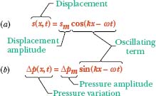
Fig. 17-6 (a) The displacement function and (b) the pressure-variation function of a traveling sound wave consist of an amplitude and an oscillating term.
Consider the thin element of air of thickness Δx shown in Fig. 17-5b. As the wave travels through this portion of the tube, the element of air oscillates left and right in simple harmonic motion about its equilibrium position. Thus, the oscillations of each air element due to the traveling sound wave are like those of a string element due to a transverse wave, except that the air element oscillates longitudinally rather than transversely. Because string elements oscillate parallel to the y axis, we write their displacements in the form y(x, t). Similarly, because air elements oscillate parallel to the x axis, we could write their displacements in the confusing form x(x, t), but we shall use s(x, t) instead.
To show that the displacements s(x, t) are sinusoidal functions of x and t, we can use either a sine function or a cosine function. In this lesson we use a cosine function, writing

Figure 17-6a labels the various parts of this equation. In it, sm is the displacement amplitude—that is, the maximum displacement of the air element to either side of its equilibrium position (see Fig. 17-5b). The angular wave number k, angular frequency ω, frequency f, wavelength λ, speed ν, and period T for a sound (longitudinal) wave are defined and interrelated exactly as for a transverse wave, except that λ is now the distance (again along the direction of travel) in which the pattern of compression and expansion due to the wave begins to repeat itself (see Fig. 17-5a). (We assume sm is much less than λ.)
As the wave moves, the air pressure at any position x in Fig. 17-5a varies sinusoidally, as we prove next. To describe this variation we write

Figure 17-6b labels the various parts of this equation. A negative value of Δp in Eq. 17-14 corresponds to an expansion of the air, and a positive value to a compression. Here Δpm is the pressure amplitude, which is the maximum increase or decrease in pressure due to the wave; Δpm is normally very much less than the pressure p present when there is no wave. As we shall prove, the pressure amplitude Δpm is related to the displacement amplitude sm in Eq. 17-13 by

Figure 17-7 shows plots of Eqs. 17-13 and 17-14 at t = 0, with time, the two curves would move rightward along the horizontal axes. Notes that the displacement and pressure variation are π/2 rad (or 90°) out of phase. Thus, for example, the pressure variation Δp at any point along the wave is zero when the displacement there is a maximum.
![]() CHECKPOINT 1 When the oscillating air element in Fig. 17-5b is moving rightward through the point of zero displacement, is the pressure in the element at its equilibrium value, just beginning to increase, or just beginning to decrease?
CHECKPOINT 1 When the oscillating air element in Fig. 17-5b is moving rightward through the point of zero displacement, is the pressure in the element at its equilibrium value, just beginning to increase, or just beginning to decrease?
Derivation of Eqs. 17-14 and 17-15
Figure 17-5b shows an oscillating element of air of cross-sectional area A and thickness Δx, with its center displaced from its equilibrium position by distance s. From Eq. 17-2 we can write, for the pressure variation in the displaced element,
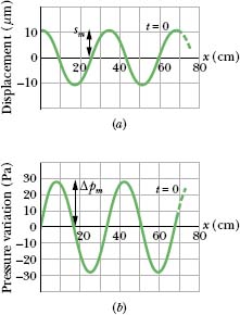
Fig. 17-7 (a) A plot of the displacement function (Eq. 17-13) for t = 0. (b) A similar plot of the pressure-variation function (Eq. 17-14). Both plots are for a 1000 Hz sound wave whose pressure amplitude is at the threshold of pain; see Sample Problem 17-2.
The quantity V in Eq. 17-16 is the volume of the element, given by

The quantity ΔV in Eq. 17-16 is the change in volume that occurs when the element is displaced. This volume change comes about because the displacements of the two faces of the element are not quite the same, differing by some amount Δs. Thus, we can write the change in volume as

Substituting Eqs. 17-17 and 17-18 into Eq. 17-16 and passing to the differential limit yield
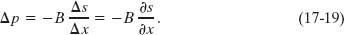
The symbols ∂ indicate that the derivative in Eq. 17-19 is a partial derivative, which tells us how s changes with x when the time t is fixed. From Eq. 17-13 we then have, treating t as a constant,

Substituting this quantity for the partial derivative in Eq. 17-19 yields

Setting Δpm = Bksm, this yields Eq. 17-14, which we set out to prove.
Using Eq. 17-3, we can now write

Equation 17-15, which we also wanted to prove, follows at once if we substitute ω/ν for k from Eq. 16-13.
The maximum pressure amplitude Δpm that the human ear can tolerate in loud sounds is about 28 Pa (which is very much less than the normal air pressure of about 105 Pa). What is the displacement amplitude sm for such a sound in air of density ρ = 1.21 kg/m3, at a frequency of 1000 Hz and a speed of 343 m/s?
Solution: The Key Idea is that the displacement amplitude sm of a sound wave is related to the pressure amplitude Δpm of the wave according to Eq. 17-15. Solving that equation for sm yields
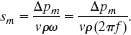
Substituting known data then gives us
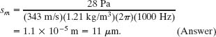
That is only about one-seventh the thickness of this page. Obviously, the displacement amplitude of even the loudest sound that the ear can tolerate is very small.
The pressure amplitude Δpm for the faintest detectable sound at 1000 Hz is 2.8 × 10⁻⁵ Pa. Proceeding as above leads to sm = 1.1 × 10⁻¹¹ m or 11 pm, which is about one-tenth the radius of a typical atom. The ear is indeed a sensitive detector of sound waves.
Leave a Reply