We turn now to a class of simple harmonic oscillators in which the springiness is associated with the gravitational force rather than with the elastic properties of a twisted wire or a compressed or stretched spring.
The Simple Pendulum
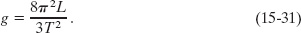
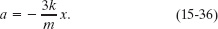
If you hang an apple at the end of a long thread fixed at its upper end and then set the apple swinging back and forth a small distance, you easily see that the apple’s motion is periodic. Is it, in fact, simple harmonic motion? If so, what is the period T? To answer, we consider a simple pendulum, which consists of a particle of mass m (called the bob of the pendulum) suspended from one end of an unstretchable, massless string of length L that is fixed at the other end, as in Fig. 15-9a. The bob is free to swing back and forth in the plane of the page, to the left and right of a vertical line through the pendulum’s pivot point.
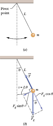
Fig. 15-9 (a) A simple pendulum. (b) The forces acting on the bob are the gravitational force ![]() and the force
and the force ![]() from the string. The tangential component Fg sin θ of the gravitational force is a restoring force that tends to bring the pendulum back to its central position.
from the string. The tangential component Fg sin θ of the gravitational force is a restoring force that tends to bring the pendulum back to its central position.
The forces acting on the bob are the force ![]() from the string and the gravitational force
from the string and the gravitational force ![]() , as shown in Fig. 15-9b, where the string makes an angle θ with the vertical. We resolve
, as shown in Fig. 15-9b, where the string makes an angle θ with the vertical. We resolve ![]() into a radial component Fg cos θ and a component Fg sin θ that is tangent to the path taken by the bob. This tangential component produces a restoring torque about the pendulum’s pivot point because the component always acts opposite the displacement of the bob so as to bring the bob back toward its central location. That location is called the equilibrium position (θ = 0) because the pendulum would be at rest there were it not swinging.
into a radial component Fg cos θ and a component Fg sin θ that is tangent to the path taken by the bob. This tangential component produces a restoring torque about the pendulum’s pivot point because the component always acts opposite the displacement of the bob so as to bring the bob back toward its central location. That location is called the equilibrium position (θ = 0) because the pendulum would be at rest there were it not swinging.
From Eq. 10-41 (τ = r⊥F), we can write this restoring torque as

where the minus sign indicates that the torque acts to reduce θ and L is the moment arm of the force component Fg sin θ about the pivot point. Substituting Eq. 15-24 into Eq. 10-44 (τ = Iα) and then substituting mg as the magnitude of Fg, we obtain

where I is the pendulum’s rotational inertia about the pivot point and α is its angular acceleration about that point.
We can simplify Eq. 15-25 if we assume the angle θ is small, for then we can approximate sin θ with θ (expressed in radian measure). (As an example, if θ = 5.00° = 0.0873 rad, then sin θ = 0.0872, a difference of only about 0.1%.) With that approximation and some rearranging, we then have
This equation is the angular equivalent of Eq. 15-8, the hallmark of SHM. It tells us that the angular acceleration α of the pendulum is proportional to the angular displacement θ but opposite in sign. Thus, as the pendulum bob moves to the right, as in Fig. 15-9a, its acceleration to the left increases until the bob stops and begins moving to the left. Then, when it is to the left of the equilibrium position, its acceleration to the right tends to return it to the right, and so on, as it swings back and forth in SHM. More precisely, the motion of a simple pendulum swinging through only small angles is approximately SHM. We can state this restriction to small angles another way: The angular amplitude θm of the motion (the maximum angle of swing) must be small.
Comparing Eqs. 15-26 and Eq. 15-8, we see that the angular frequency of the pendulum is ![]() . Next, if we substitute this expression for ω into Eq. 15-5 (ω = 2π/T), we see that the period of the pendulum may be written as
. Next, if we substitute this expression for ω into Eq. 15-5 (ω = 2π/T), we see that the period of the pendulum may be written as
All the mass of a simple pendulum is concentrated in the mass m of the particle like bob, which is at radius L from the pivot point. Thus, we can use Eq. 10-33 (I = mr2) to write I = mL2 for the rotational inertia of the pendulum. Substituting this into Eq. 15-27 and simplifying then yield

as a simpler expression for the period of a simple pendulum swinging through only small angles. (We assume small-angle swinging in this lesson.)
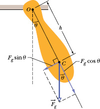
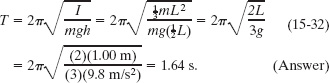
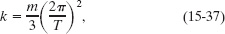
Fig. 15-10 A physical pendulum. The restoring torque is hFg sin θ. When θ = 0, center of mass C hangs directly below pivot point O.
The Physical Pendulum
A real pendulum, usually called a physical pendulum, can have a complicated distribution of mass, much different from that of a simple pendulum. Does a physical pendulum also undergo SHM? If so, what is its period?
Figure 15-10 shows an arbitrary physical pendulum displaced to one side by angle θ. The gravitational force ![]() acts at its center of mass C, at a distance h from the pivot point O. Comparison of Figs. 15-10 and 15-9b reveals only one important difference between an arbitrary physical pendulum and a simple pendulum. For a physical pendulum the restoring component Fg sin θ of the gravitational force has a moment arm of distance h about the pivot point, rather than of string length L. In all other respects, an analysis of the physical pendulum would duplicate our analysis of the simple pendulum up through Eq. 15-27. Again, (for small θm) we would find that the motion is approximately SHM.
acts at its center of mass C, at a distance h from the pivot point O. Comparison of Figs. 15-10 and 15-9b reveals only one important difference between an arbitrary physical pendulum and a simple pendulum. For a physical pendulum the restoring component Fg sin θ of the gravitational force has a moment arm of distance h about the pivot point, rather than of string length L. In all other respects, an analysis of the physical pendulum would duplicate our analysis of the simple pendulum up through Eq. 15-27. Again, (for small θm) we would find that the motion is approximately SHM.
If we replace L with h in Eq. 15-27, we can write the period as

As with the simple pendulum, I is the rotational inertia of the pendulum about O. However, now I is not simply mL2 (it depends on the shape of the physical pendulum), but it is still proportional to m.
A physical pendulum will not swing if it pivots at its center of mass. Formally, this corresponds to putting h = 0 in Eq. 15-29. That equation then predicts T → ∞, which implies that such a pendulum will never complete one swing.
Corresponding to any physical pendulum that oscillates about a given pivot point O with period T is a simple pendulum of length L0 with the same period T. We can find L0 with Eq. 15-28. The point along the physical pendulum at distance L0 from point O is called the center of oscillation of the physical pendulum for the given suspension point.
Measuring g
We can use a physical pendulum to measure the free-fall acceleration g at a particular location on Earth’s surface. (Countless thousands of such measurements have been made during geophysical prospecting.)
To analyze a simple case, take the pendulum to be a uniform rod of length L, suspended from one end. For such a pendulum, h in Eq. 15-29, the distance between the pivot point and the center of mass, is ![]() . Table 10-2e tells us that the rotational inertia of this pendulum about a perpendicular axis through its center of mass is
. Table 10-2e tells us that the rotational inertia of this pendulum about a perpendicular axis through its center of mass is ![]() . From the parallel-axis theorem of Eq. 10-36 (I = Icom + Mh2), we then find that the rotational inertia about a perpendicular axis through one end of the rod is
. From the parallel-axis theorem of Eq. 10-36 (I = Icom + Mh2), we then find that the rotational inertia about a perpendicular axis through one end of the rod is

If we put ![]() and
and ![]() in Eq. 15-29 and solve for g, we find
in Eq. 15-29 and solve for g, we find
Thus, by measuring L and the period T, we can find the value of g at the pendulum’s location. (If precise measurements are to be made, a number of refinements are needed, such as swinging the pendulum in an evacuated chamber.)
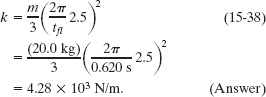
In Fig. 15-11a, a meter stick swings about a pivot point at one end, at distance h from the stick’s center of mass.
(a) What is the period of oscillation T?
Solution: One Key Idea here is that the stick is not a simple pendulum because its mass is not concentrated in a bob at the end opposite the pivot point—so the stick is a physical pendulum. Then its period is given by Eq. 15-29, for which we need the rotational inertia I of the stick about the pivot point. We can treat the stick as a uniform rod of length L and mass m. Then Eq. 15-30 tells us that ![]() , and the distance h in Eq. 15-29 is
, and the distance h in Eq. 15-29 is ![]() . Substituting these quantities into Eq. 15-29, we find
. Substituting these quantities into Eq. 15-29, we find
Note the result is independent of the pendulum’s mass m.
(b) What is the distance L0 between the pivot point O of the stick and the center of oscillation of the stick?
Solution: The Key Idea here is that we want the length L0 of the simple pendulum (drawn in Fig. 15-11b) that has the same period as the physical pendulum (the stick) of Fig. 15-11a. Setting Eqs. 15-28 and 15-32 equal yields

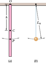
Fig. 15-11 (a) A meter stick suspended from one end as a physical pendulum. (b) A simple pendulum whose length L0 is chosen so that the periods of the two pendulums are equal. Point P on the pendulum of (a) marks the center of oscillation.
You can see by inspection that

In Fig. 15-11a, point P marks this distance from suspension point O. Thus, point P is the stick’s center of oscillation for the given suspension point.
![]() CHECKPOINT 4 Three physical pendulums, of masses m0, 2m0, and 3m0, have the same shape and size and are suspended at the same point. Rank the masses according to the periods of the pendulums, greatest first.
CHECKPOINT 4 Three physical pendulums, of masses m0, 2m0, and 3m0, have the same shape and size and are suspended at the same point. Rank the masses according to the periods of the pendulums, greatest first.
A competition diving board sits on a fulcrum about one-third of the way out from the fixed end of the board (Fig. 15-12a). In a running dive, a diver takes three quick steps along the board, out past the fulcrum so as to rotate the board’s free end downward. As the board rebounds back through the horizontal, the diver leaps upward and toward the board’s free end (Fig. 15-12b). A skilled diver trains to land on the free end just as the board has completed 2.5 oscillations during the leap. With such timing, the diver lands as the free end is moving downward with greatest speed (Fig. 15-12c). The landing then drives the free end down substantially, and the rebound catapults the diver high into the air.
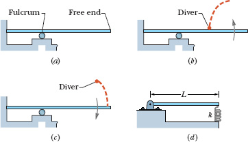
Fig. 15-12 (a) A diving board. (b) The diver leaps upward and forward as the board moves through the horizontal. (c) The diver lands 2.5 oscillations later. (d) A spring-oscillator model of the oscillating board.
Figure 15-12d shows a simple but realistic model of a competition board. The board section beyond the fulcrum is treated as a stiff rod of length L that can rotate about a hinge at the fulcrum, compressing an (imaginary) spring under the board’s free end. If the rod’s mass is m = 20.0 kg and the diver’s leap lasts tfl = 0.620 s, what spring constant k is required of the spring for a proper landing?
Solution: Because a spring is involved, we might guess that the oscillations are SHM, but we shall not assume that. Instead, we use the following Key Idea: If the rod is in SHM, then the acceleration and displacement of the oscillating end of the rod must be related by an expression in the form of Eq. 15-8 (a = −ω2x). If so, we shall be able to find ω and then the desired k from the expression. Let us check by finding the relation between the acceleration and displacement of the rod’s right end.
Because the rod rotates about the hinge as the free end oscillates, we are concerned with a torque ![]() on the rod about the hinge. That torque is due to the force
on the rod about the hinge. That torque is due to the force ![]() on the rod from the spring. Because
on the rod from the spring. Because ![]() varies with time,
varies with time, ![]() must also. However, at any given instant we can relate the magnitudes of
must also. However, at any given instant we can relate the magnitudes of ![]() and
and ![]() with Eq. 10-39 (τ = rF sin
with Eq. 10-39 (τ = rF sin ![]() ). Here we have
). Here we have

where L is the moment arm of force ![]() and 90° is the angle between the moment arm and the force’s line of action. Combining Eq. 15-33 with Eq. 10-44 (τ = Iα) gives us
and 90° is the angle between the moment arm and the force’s line of action. Combining Eq. 15-33 with Eq. 10-44 (τ = Iα) gives us

where I is the rod’s rotational inertia about the hinge and α is its angular acceleration about that point. From Eq. 15-30, the rod’s rotational inertia I is ![]() .
.
Now let us mentally erect a vertical x axis through the oscillating right end of the rod, with the positive direction upward. Then the force on the right end of the rod from the spring is F = −kx, where x is the vertical displacement of the right end.
Substituting these expressions for I and F into Eq. 15-34 gives us
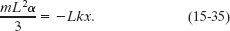
We now have a mixture of linear displacement x (vertically) and rotational acceleration α (about the hinge). We can replace α in Eq. 15-35 with the (linear) acceleration a along the x axis by substituting according to Eq. 10-22 (at = αr) for tangential acceleration. Here the tangential acceleration is a and the radius of rotation r is L, so α = a/L. With that substitution, Eq. 15-35 becomes

which yields
Equation 15-36 is, in fact, of the same form as Eq. 15-8 (a = −ω2x). Therefore, the rod does indeed undergo SHM, and comparison of Eqs. 15-36 and 15-8 shows that

Solving for k and substituting for ω from Eq. 15-5 (ω = 2π/T) give us
where T is the period of the board’s oscillation. We want the time of flight tfl to last for 2.5 oscillations of the board and thus also for 2.5 oscillations of our rod. Thus we want tfl = 2.5T. Substituting this and given data into Eq. 15-37 leads to
This is the effective spring constant k of the diving board.
From Eq. 15-38, we see that a diver with a longer flight time tfl requires a smaller spring constant k in order to land at the proper instant at the end of the board. The value of k can be increased by moving the fulcrum toward the free end or decreased by moving it in the opposite direction. A skilled diver trains to leap with a certain flight time tfl and knows how to set the fulcrum position accordingly.
Leave a Reply