Figure 15-1a shows a sequence of “snapshots” of a simple oscillating system, a particle moving repeatedly back and forth about the origin of an x axis. In this section we simply describe the motion. Later, we shall discuss how to attain such motion.
One important property of oscillatory motion is its frequency, or number of oscillations that are completed each second. The symbol for frequency is f, and its SI unit is the hertz (abbreviated Hz), where

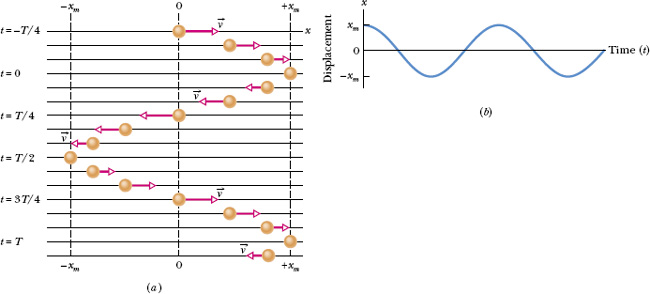
Fig. 15-1 (a) A sequence of “snapshots” (taken at equal time intervals) showing the position of a particle as it oscillates back and forth about the origin of an x axis, between the limits +xm and −xm. The vector arrows are scaled to indicate the speed of the particle. The speed is maximum when the particle is at the origin and zero when it is at ±xm. If the time t is chosen to be zero when the particle is at +xm, then the particle returns to +xm at t = T, where T is the period of the motion. The motion is then repeated. (b) A graph of x as a function of time for the motion of (a).
Related to the frequency is the period T of the motion, which is the time for one complete oscillation (or cycle); that is,

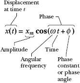
Fig. 15-2 A handy reference to the quantities in Eq. 15-3 for simple harmonic motion.
Any motion that repeats itself at regular intervals is called periodic motion or harmonic motion. We are interested here in motion that repeats itself in a particular way—namely, like that in Fig. 15-1a. For such motion the displacement x of the particle from the origin is given as a function of time by

in which xm, ω, and ![]() are constants. This motion is called simple harmonic motion (SHM), a term that means the periodic motion is a sinusoidal function of time. Equation 15-3, in which the sinusoidal function is a cosine function, is graphed in Fig. 15-1b. (You can get that graph by rotating Fig. 15-1a counterclockwise by 90° and then connecting the successive locations of the particle with a curve.) The quantities that determine the shape of the graph are displayed in Fig. 15-2 with their names. We now shall define those quantities.
are constants. This motion is called simple harmonic motion (SHM), a term that means the periodic motion is a sinusoidal function of time. Equation 15-3, in which the sinusoidal function is a cosine function, is graphed in Fig. 15-1b. (You can get that graph by rotating Fig. 15-1a counterclockwise by 90° and then connecting the successive locations of the particle with a curve.) The quantities that determine the shape of the graph are displayed in Fig. 15-2 with their names. We now shall define those quantities.
The quantity xm, called the amplitude of the motion, is a positive constant whose value depends on how the motion was started. The subscript m stands for maximum because the amplitude is the magnitude of the maximum displacement of the particle in either direction. The cosine function in Eq. 15-3 varies between the limits ±1; so the displacement x(t) varies between the limits ±xm.
The time-varying quantity ![]() in Eq. 15-3 is called the phase of the motion, and the constant
in Eq. 15-3 is called the phase of the motion, and the constant ![]() is called the phase constant (or phase angle). The value of
is called the phase constant (or phase angle). The value of ![]() depends on the displacement and velocity of the particle at time t = 0. For the x(t) plots of Fig. 15-3a, the phase constant
depends on the displacement and velocity of the particle at time t = 0. For the x(t) plots of Fig. 15-3a, the phase constant ![]() is zero.
is zero.
To interpret the constant ω, called the angular frequency of the motion, we first note that the displacement x(t) must return to its initial value after one period T of the motion; that is, x(t) must equal x(t + T) for all t. To simplify this analysis, let us put ![]() in Eq. 15-3. From that equation we then can write
in Eq. 15-3. From that equation we then can write

The cosine function first repeats itself when its argument (the phase) has increased by 2π rad; so Eq. 15-4 gives us
ω(t + T) = ωt + 2π
or
ωT = 2π.

Fig. 15-3 In all three cases, the blue curve is obtained from Eq. 15-3 with ![]() . (a) The red curve differs from the blue curve only in that the red-curve amplitude
. (a) The red curve differs from the blue curve only in that the red-curve amplitude ![]() is greater (the red-curve extremes of displacement are higher and lower). (b) The red curve differs from the blue curve only in that the red-curve period is T′ = T/2 (the red curve is compressed horizontally). (c) The red curve differs from the blue curve only in that for the red-curve
is greater (the red-curve extremes of displacement are higher and lower). (b) The red curve differs from the blue curve only in that the red-curve period is T′ = T/2 (the red curve is compressed horizontally). (c) The red curve differs from the blue curve only in that for the red-curve ![]() rad rather than zero (the negative value of
rad rather than zero (the negative value of ![]() shifts the red curve to the right).
shifts the red curve to the right).
Thus, from Eq. 15-2 the angular frequency is

The SI unit of angular frequency is the radian per second. (To be consistent, then, ![]() must be in radians.) Figure 15-3 compares x(t) for two simple harmonic motions that differ either in amplitude, in period (and thus in frequency and angular frequency), or in phase constant.
must be in radians.) Figure 15-3 compares x(t) for two simple harmonic motions that differ either in amplitude, in period (and thus in frequency and angular frequency), or in phase constant.
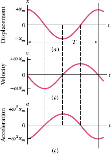
Fig. 15-4 (a) The displacement x(t) of a particle oscillating in SHM with phase angle ![]() equal to zero. The period T marks one complete oscillation. (b) The velocity v(t) of the particle. (c) The acceleration a(t) of the particle.
equal to zero. The period T marks one complete oscillation. (b) The velocity v(t) of the particle. (c) The acceleration a(t) of the particle.
![]() CHECKPOINT 1 A particle undergoing simple harmonic oscillation of period T (like that in Fig. 15-1) is at −xm at time t = 0. Is it at −xm, at +xm, at 0, between −xm and 0, or between 0 and +xm when (a) t = 2.00T, (b) t = 3.50T, and (c) t = 5.25T?
CHECKPOINT 1 A particle undergoing simple harmonic oscillation of period T (like that in Fig. 15-1) is at −xm at time t = 0. Is it at −xm, at +xm, at 0, between −xm and 0, or between 0 and +xm when (a) t = 2.00T, (b) t = 3.50T, and (c) t = 5.25T?
The Velocity of SHM
By differentiating Eq. 15-3, we can find an expression for the velocity of a particle moving with simple harmonic motion; that is,
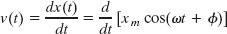

Figure 15-4a is a plot of Eq. 15-3 with ![]() . Figure 15-4b shows Eq. 15-6, also with
. Figure 15-4b shows Eq. 15-6, also with ![]() . Analogous to the amplitude xm in Eq. 15-3, the positive quantity ωxm in Eq. 15-6 is called the velocity amplitude vm. As you can see in Fig. 15-4b, the velocity of the oscillating particle varies between the limits ±vm = ±ωxm. Note also in that figure that the curve of v(t) is shifted (to the left) from the curve of x(t) by one-quarter period; when the magnitude of the displacement is greatest (that is, x(t) = xm), the magnitude of the velocity is least (that is, v(t) = 0). When the magnitude of the displacement is least (that is, zero), the magnitude of the velocity is greatest (that is, vm = ωxm).
. Analogous to the amplitude xm in Eq. 15-3, the positive quantity ωxm in Eq. 15-6 is called the velocity amplitude vm. As you can see in Fig. 15-4b, the velocity of the oscillating particle varies between the limits ±vm = ±ωxm. Note also in that figure that the curve of v(t) is shifted (to the left) from the curve of x(t) by one-quarter period; when the magnitude of the displacement is greatest (that is, x(t) = xm), the magnitude of the velocity is least (that is, v(t) = 0). When the magnitude of the displacement is least (that is, zero), the magnitude of the velocity is greatest (that is, vm = ωxm).
The Acceleration of SHM
Knowing the velocity v(t) for simple harmonic motion, we can find an expression for the acceleration of the oscillating particle by differentiating once more. Thus, we have, from Eq. 15-6,

Figure 15-4c is a plot of Eq. 15-7 for the case ![]() . The positive quantity ω2xm in Eq. 15-7 is called the acceleration amplitude am; that is, the acceleration of the particle varies between the limits ±am = ±ω2xm, as Fig. 15-4c shows. Note also that the acceleration curve a(t) is shifted (to the left) by
. The positive quantity ω2xm in Eq. 15-7 is called the acceleration amplitude am; that is, the acceleration of the particle varies between the limits ±am = ±ω2xm, as Fig. 15-4c shows. Note also that the acceleration curve a(t) is shifted (to the left) by ![]() relative to the velocity curve v(t).
relative to the velocity curve v(t).
We can combine Eqs. 15-3 and 15-7 to yield

which is the hallmark of simple harmonic motion:
![]() In SHM, the acceleration is proportional to the displacement but opposite in sign, and the two quantities are related by the square of the angular frequency.
In SHM, the acceleration is proportional to the displacement but opposite in sign, and the two quantities are related by the square of the angular frequency.
Thus, as Fig. 15-4 shows, when the displacement has its greatest positive value, the acceleration has its greatest negative value, and conversely. When the displacement is zero, the acceleration is also zero.
PROBLEM – SOLVING TACTICS
TACTIC 1: Phase Angles
Note the effect of the phase angle ![]() on a plot of x(t). When
on a plot of x(t). When ![]() , x(t) has a graph like that in Fig. 15-4a, a typical cosine curve. Increasing
, x(t) has a graph like that in Fig. 15-4a, a typical cosine curve. Increasing ![]() shifts the curve leftward along the t axis. (You might remember this with the symbol
shifts the curve leftward along the t axis. (You might remember this with the symbol ![]() , where the up arrow indicates an increase in
, where the up arrow indicates an increase in ![]() and the left arrow indicates the resulting shift in the curve.) Decreasing
and the left arrow indicates the resulting shift in the curve.) Decreasing ![]() shifts the curve rightward, as in Fig. 15-3c for
shifts the curve rightward, as in Fig. 15-3c for ![]() .
.
Two plots of SHM with different phase angles are said to have a phase difference; each is said to be phase-shifted from the other, or out of phase with the other. The curves in Fig. 15-3c, for example, have a phase difference of π/4 rad.
Because SHM repeats after each period T and the cosine function repeats after each 2π rad, one period T represents a phase difference of 2π rad. In Fig. 15-4, x(t) is phase-shifted to the right from v(t) by one-quarter period, or −π/2 rad; it is shifted to the right from a(t) by one-half period, or −π rad. A phase shift of 2π rad causes a curve of SHM to coincide with itself; that is, it looks unchanged.
Leave a Reply